Real Estate¶

Model Set Up¶

Link to the dataset
Dataset original source
Complete example code
Determine the price of houses by their features.
The market historical data set of real estate valuation are collected from Sindian Dist., New Taipei City, Taiwan.

import pandas as pd

data = pd.read_csv(r'data/data.csv')
data.drop(columns=['No'], inplace=True)
data.columns = [' '.join(col.split(' ')[1:]) for col in data.columns]
data.rename(
    columns={
        'distance to the nearest MRT station': 'MRT station distance',
        'number of convenience stores': 'stores number',
        'house price of unit area': 'house price'
    },
    inplace=True
)

Data exploration:

import matplotlib.pyplot as plt

pd.plotting.scatter_matrix(frame=data, figsize=(10, 10))

plt.tight_layout()

plt.show()

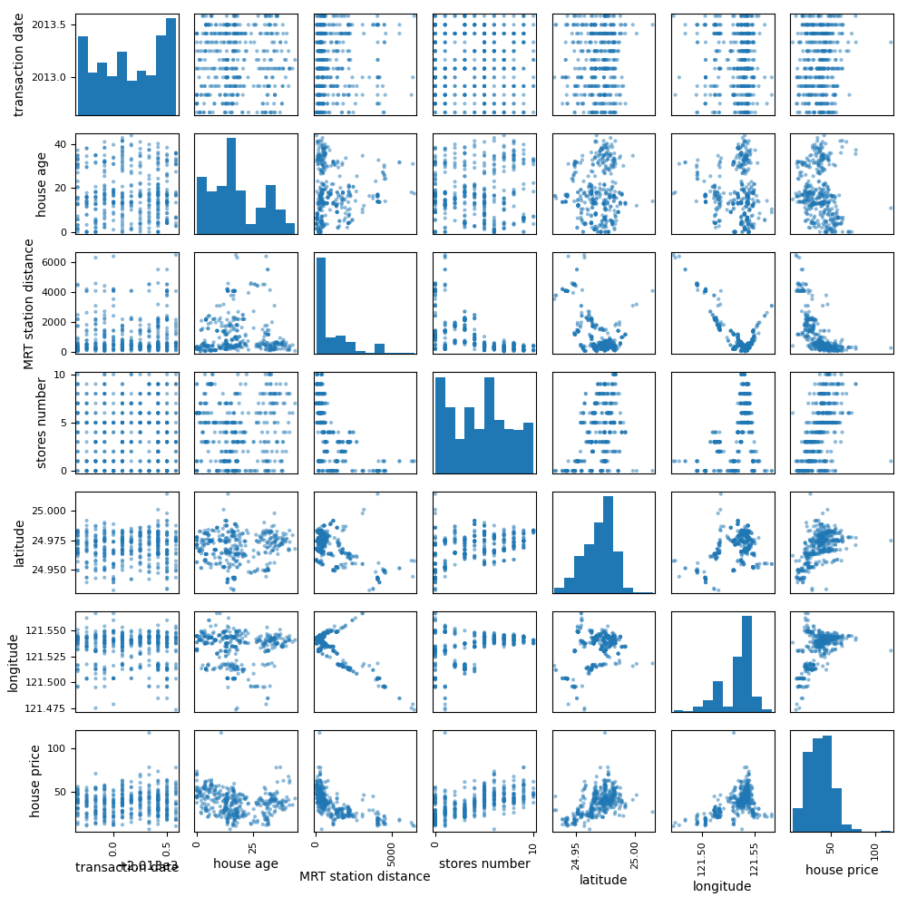
The scatterplot shows no strong correlation among regressors.
There are two outliers in house price, one under 8 and the other over 115, that do not follow the rest of distributions. For this reason, the outliers are removed.
house price and MRT station distance are not normally distributed: data are skewed toward high values. For this reason, these columns are transformed to log-scale:

import numpy as np

data = data[(data['house price'] > 8) & (data['house price'] < 115)]
data['log house price'] = np.log(data['house price'])
data['log MRT station distance'] = np.log(data['MRT station distance'])

Set up a linear regression model, considering transaction date, house age, log MRT station distance, stores number, latitude and longitude as the regressors and log house price as the response variable.
Using non-informative priors for regressors and variance:

from baypy.model import LinearModel
import baypy as bp

model = LinearModel()
model.data = data
model.response_variable = 'log house price'
model.priors = {
    'intercept': {'mean': 0, 'variance': 1e6},
    'transaction date': {'mean': 0, 'variance': 1e6},
    'house age': {'mean': 0, 'variance': 1e6},
    'log MRT station distance': {'mean': 0, 'variance': 1e6},
    'stores number': {'mean': 0, 'variance': 1e6},
    'latitude': {'mean': 0, 'variance': 1e6},
    'longitude': {'mean': 0, 'variance': 1e6},
    'variance': {'shape': 1, 'scale': 1e-6}
}

See LinearModel for more information on this class and its attributes and methods.

Sampling¶

Run the regression sampling on 3 Markov chains, with 1000 iterations per each chain and discarding the first 50 burn-in draws:

from baypy.regression import LinearRegression

LinearRegression.sample(
    model=model,
    n_iterations=1000, 
    burn_in_iterations=50,
    n_chains=3,
    seed=137
)

See LinearRegression for more information on this class and its attributes and methods.

Convergence Diagnostics¶

Asses the model convergence diagnostics:

bp.diagnostics.effective_sample_size(posteriors=model.posteriors)

                       intercept  transaction date  house age  log MRT station distance  stores number  latitude  longitude  variance
Effective Sample Size    2767.17           2833.16    2548.86                   2877.61        2630.62   2770.24    2753.23   2778.72

bp.diagnostics.autocorrelation_summary(posteriors=model.posteriors)

        intercept  transaction date  house age  log MRT station distance  stores number  latitude  longitude  variance
Lag 0    1.000000          1.000000   1.000000                  1.000000       1.000000  1.000000   1.000000  1.000000
Lag 1   -0.009739         -0.000259   0.000069                 -0.027052       0.001308  0.009574  -0.028492  0.034033
Lag 5   -0.004870         -0.010960  -0.017678                  0.010558       0.003372 -0.004647  -0.003221 -0.029635
Lag 10   0.014359          0.003361   0.009231                  0.013320      -0.012113 -0.017253   0.016727 -0.000938
Lag 30  -0.000886          0.031398  -0.030163                 -0.027021       0.004524  0.000075  -0.034411 -0.043168

bp.diagnostics.autocorrelation_plot(posteriors=model.posteriors)

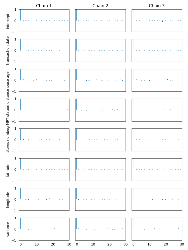
See effective_sample_size, autocorrelation_summary and autocorrelation_plot for more details on diagnostics functions.
All diagnostics show a low correlation, indicating the chains converged to the stationary distribution.

Posteriors Analysis¶

Asses posterior analysis:

bp.analysis.trace_plot(posteriors=model.posteriors)

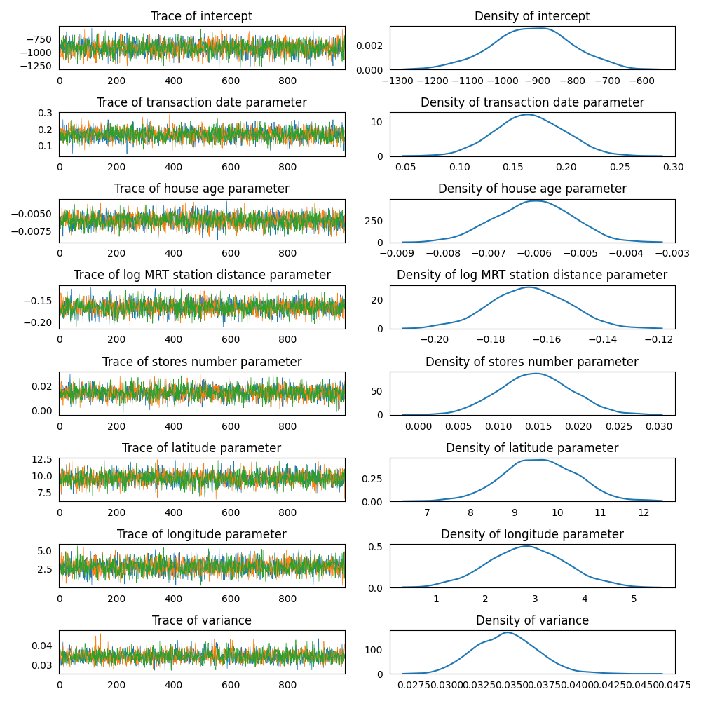
Traces are good, indicating draws from the stationary distribution.

bp.analysis.residuals_plot(model=model)

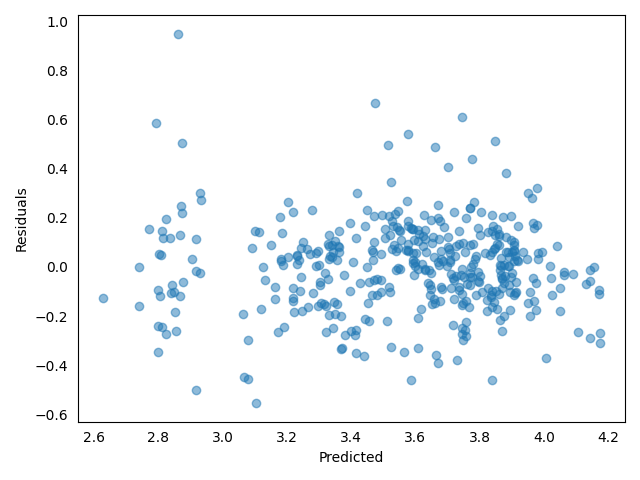
Also, the residuals plot is good: no evidence for patterns, shapes or outliers.

bp.analysis.summary(posteriors=model.posteriors)

Number of chains:           3
Sample size per chian:   1000

Empirical mean, standard deviation, 95% HPD interval for each variable:

                                Mean          SD      HPD min     HPD max
intercept                -914.144001  114.532293 -1140.625297 -689.444488
transaction date            0.165923    0.032401     0.102919    0.227775
house age                  -0.006024    0.000831    -0.007647   -0.004449
log MRT station distance   -0.166081    0.013939    -0.192367   -0.137433
stores number               0.014637    0.004559     0.005655    0.023409
latitude                    9.593946    0.851219     7.979301   11.251111
longitude                   2.840717    0.797554     1.193730    4.361885
variance                    0.034584    0.002446     0.029867    0.039150

Quantiles for each variable:

                                 2.5%         25%         50%         75%       97.5%
intercept                -1145.639542 -989.823076 -913.067376 -837.985390 -693.822181
transaction date             0.104168    0.144264    0.165367    0.187846    0.229589
house age                   -0.007658   -0.006587   -0.006004   -0.005448   -0.004454
log MRT station distance    -0.194091   -0.175519   -0.166026   -0.156556   -0.138945
stores number                0.005802    0.011556    0.014616    0.017608    0.023622
latitude                     7.933698    9.032735    9.583895   10.176279   11.219930
longitude                    1.262242    2.303130    2.840166    3.366287    4.466213
variance                     0.030052    0.032863    0.034565    0.036164    0.039478

See trace_plot, residuals_plot and summary for more details on analysis functions.
The summary reports a statistical evidence for:

positive effect of transaction date: \(1\) month increase would result in \(e^{\frac{0.165923}{12}} - 1 = 1.4\%\) percent increase in house price
negative effect of house age: \(1\) year increase would result in \(e^{-0.006024} - 1 = -0.6\%\) percent decrease in house price
negative effect of log MRT station distance: \(10\%\) percent increase in MRT station distance would result in \(1.10^{-0.166081} - 1 = -1.57\%\) percent decrease in house price
positive effect of stores number: \(1\) store increase would result in \(e^{0.014637} - 1 = 1.47\%\) percent increase in house price
positive effect of latitude: \(1'\) increase would result in \(e^{\frac{9.593946}{60}} - 1 = 17.3\%\) percent increase house price
positive effect of longitude: \(1'\) increase would result in \(e^{\frac{2.840717}{60}} - 1 = 4.85\%\) percent increase in house price

The combined effect of latitude and longitude suggest that the north-east of New Taipei City is the most expensive area, while the south-west is the cheapest area.