Model Set Up

Link to the dataset
Unfortunately, the database original source does not report the units on each variable.
Complete example code
Determine the effect that the independent variables biking and smoking have on the dependent variable heart disease using a multiple linear regression model.

import pandas as pd

data = pd.read_csv(r'data/data.csv')

Set up a multiple linear regression model, considering biking and smoking as regressors and heart disease as the response variable. Use non-informative priors for regressors and variance:

from baypy.model import LinearModel
import baypy as bp

model = LinearModel()

model.data = data
model.response_variable = 'heart disease'
model.priors = {
    'intercept': {'mean': 0, 'variance': 1e6},
    'biking': {'mean': 0, 'variance': 1e9},
    'smoking': {'mean': 0, 'variance': 1e9},
    'variance': {'shape': 1, 'scale': 1e-9}
}

See LinearModel for more information on this class and its attributes and methods.

Sampling

Run the regression sampling on 3 Markov chains, with 500 iterations per each chain and discarding the first 50 burn-in draws:

from baypy.regression import LinearRegression

LinearRegression.sample(
    model=model,
    n_iterations=500, 
    burn_in_iterations=50,
    n_chains=3,
    seed=137
)

See LinearRegression for more information on this class and its attributes and methods.

Convergence Diagnostics

Asses the model convergence diagnostics:

bp.diagnostics.effective_sample_size(posteriors=model.posteriors)

                       intercept   biking  smoking  variance
Effective Sample Size    1389.56  1449.73  1362.26   1426.75

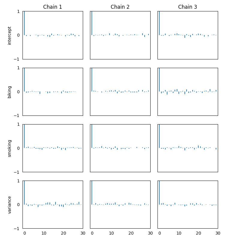
bp.diagnostics.autocorrelation_summary(posteriors=model.posteriors)

        intercept    biking   smoking  variance
Lag 0    1.000000  1.000000  1.000000  1.000000
Lag 1   -0.025015 -0.021166  0.009275 -0.021082
Lag 5    0.027681 -0.007564  0.046201  0.030989
Lag 10   0.015334  0.014290  0.043676 -0.057992
Lag 30  -0.041058 -0.008922 -0.013752 -0.040056

bp.diagnostics.autocorrelation_plot(posteriors=model.posteriors)

See effective_sample_size, autocorrelation_summary and autocorrelation_plot for more details on diagnostics functions.
All diagnostics show a low correlation, indicating the chains converged to the stationary distribution.

Posteriors Analysis

Asses posterior analysis:

bp.analysis.trace_plot(posteriors=model.posteriors)

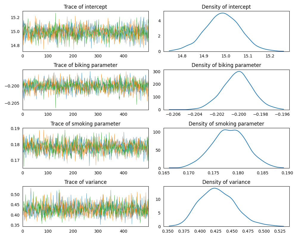
Traces are quite good, indicating draws from the stationary distribution.

bp.analysis.residuals_plot(model=model)

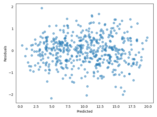
Also, the residuals plot is good: no evidence for patterns, shapes or outliers.

bp.analysis.summary(posteriors=model.posteriors)

Number of chains:           3
Sample size per chian:    500

Empirical mean, standard deviation, 95% HPD interval for each variable:

                Mean        SD    HPD min    HPD max
intercept  14.985169  0.079494  14.811145  15.126328
biking     -0.200122  0.001387  -0.203015  -0.197531
smoking     0.178261  0.003535   0.171384   0.185280
variance    0.427870  0.027745   0.374502   0.480325

Quantiles for each variable:

                2.5%        25%        50%        75%      97.5%
intercept  14.822835  14.933689  14.986087  15.039621  15.141583
biking     -0.202909  -0.201028  -0.200086  -0.199219  -0.197334
smoking     0.171140   0.175893   0.178261   0.180621   0.185169
variance    0.380265   0.408345   0.426025   0.446627   0.488800

See trace_plot, residuals_plot and summary for more details on analysis functions.
The summary reports a statistical evidence for:

• negative effect of biking: \(1\) point increase in biking would result in \(0.2\) points decrease in heart disease

• positive effect of smoking: \(1\) point increase in smoking would result \(0.18\) points increase in heart disease